Recommender System for VNDB: EDA and a Simple Content Based Model

By : Pragun Saini | 13 July 2020

Getting and loading the data

VNDB provides database dumps of specific parts of it's database like traits, tags, votes, etc as well as a complete database dump. All options are listed here. I am going to load the complete database dump so we can get all the information in one go. It is provided in the form of a PostgreSQL dump so we need to install it too. Here's how I did it on Colab.

# For postgresql setup on colab

# Install postgresql server
!sudo apt-get -y -qq update
!sudo apt-get -y -qq install postgresql
!sudo service postgresql start

# # Setup a new user `vndb`
!sudo -u postgres createuser --superuser vndb
!sudo -u postgres createdb vndb
!sudo -u postgres psql -c "ALTER USER vndb PASSWORD 'vndb'"

# Download vndb database dump
!curl -L https://dl.vndb.org/dump/vndb-db-latest.tar.zst -O

# Extract and Load data in postgresql
!sudo apt-get install zstd
!tar -I zstd -xvf vndb-db-latest.tar.zst
!PGPASSWORD=vndb psql -U vndb -h 127.0.0.1 vndb -f import.sql

To explore and work with the data, we need to import some common Python data science packages.

# SQL
import sqlalchemy

# Data Handling
import pandas as pd
import numpy as np
import sklearn
from scipy.sparse import csr_matrix, save_npz, load_npz

# Plotting
import matplotlib.pyplot as plt
import seaborn as sns
sns.set_style('whitegrid')
from wordcloud import WordCloud

And to connect to Postgres via Python we need a sqlalchemy engine.

# PostgreSQL engine
engine = sqlalchemy.create_engine(f'postgresql://vndb:vndb@localhost:5432/vndb')

Exploratory Data Analysis

As you can see getting and loading the data is easy. Now let's do some EDA on the data.

We are mainly interested in the VNs, the users, the ratings given to the VN and the tag metadata attached with the VNs.

Tags metadata

Let's focus on tags first. Users on VNDB give votes to tags related to a VN. Let's load all tags that have positive votes.

# Read all tags given to vns with vote > 0
tags_vn = pd.read_sql('Select tags.name, tags.cat from tags INNER JOIN tags_vn ON tags.id = tags_vn.tag WHERE tags_vn.vote > 0', con=engine)

# Excluding ero for some dignity
tags_vn.sample(10)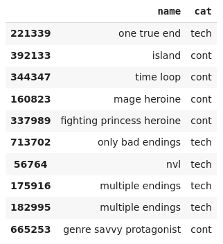

sample of tags — A glimpse of some of the tags

Upon building a word cloud of the tags based on their usage frequency, we can clearly get some intuition about the demographic of the users. Here's a link to it, because it's too explicit to put here.

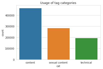
The tags themselves are divided into three categories - content, technical and ero (that's sexual content for short). You can see the usage of these categories below.

VN Ratings

Let's now explore the ratings given by users to VNs.

finished = pd.read_sql('Select uv.uid, uv.vid, uv.vote, uv.lastmod FROM ulist_vns uv INNER JOIN ulist_vns_labels uvl ON uv.uid = uvl.uid AND uv.vid = uvl.vid AND uvl.lbl = 2', con=engine)

finished = finished.dropna()
finished.sample(5)
finished["vote"].describe()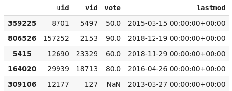

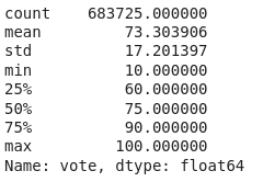
We can see that the ratings range from 10 to 100. Huh? Actually users can give votes from 1 to 10 (upto one decimal places) and these votes are multiplied by 10 as seen here.

# Plotting votes in range 1-10
sns.distplot(np.round(finished["vote"]/10), bins=10)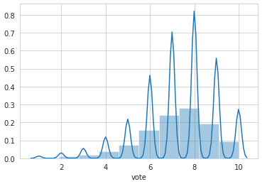

Let's print some concrete metrics about this data.

def rating_stats(df):
    print(f"Rating Count: {len(df)}")
    print(f"User Count: {len(df.uid.unique())}")
    print(f"VN Count: {len(df.vid.unique())}")
    print(f"Matrix density: {len(df)/(len(df.uid.unique()) * len(df.vid.unique()))}")
    
    user_grp = df.groupby("uid")
    user_vote_cnt = user_grp.count()["vote"]
    print(f"Max # of voted VN by a user: {user_vote_cnt.max()}")
    print(f"Min # of voted VN by a user: {user_vote_cnt.min()}")
    print(f"Average # of voted VN by a user: {user_vote_cnt.mean()}")
    
    vn_grp = df.groupby("vid")
    vn_vote_cnt = vn_grp.count()["vote"]
    print(f"Max # of users voted a VN: {vn_vote_cnt.max()}")
    print(f"Min # of users voted a VN: {vn_vote_cnt.min()}")
    print(f"Average # of users voted a VN: {vn_vote_cnt.mean()}")

rating_stats(finished)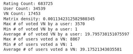

If you look at the density, it's too low. Such data is caled sparse data and is common in such ratings databases, because even though there are lot of users and items, not all users use or rate every item.

Now let's look at the user ratings distributions.

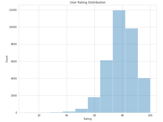
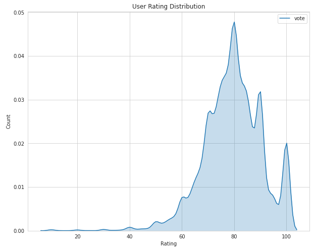
There's a tendency to vote in the region of 6-10. This can be explained, because most of the users either don't play bad VNs that could have got lower ratings, or maybe they play and drop it midway, not bothering to even rate them.

Now let's look at the opposite end, the VN ratings distribution.

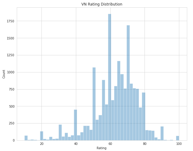
It's much more chaotic, with few VNs getting high (around 10) or low (<= 3) votes, in general the votes are pretty balanced in the middle ranges.

Let's also look at how many votes VNs actually get in general.

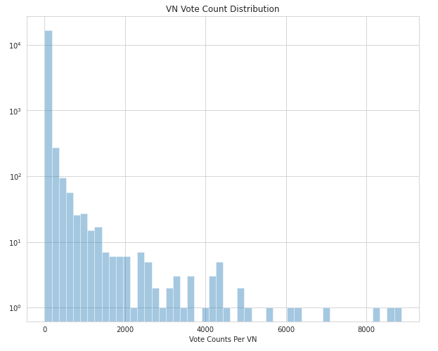
As you would have figured out yourself upon thinking, majority of votes are given to very few VNs which are probably the popular or highest rated ones.

Let's look at these highest rated VNs using their mean ratings.

# Highest Rated VNs
best_vns = finished.groupby("vid").agg(["count", "mean"])["vote"]
best_vns = best_vns.sort_values(by="mean", ascending=False)
best_vns.head()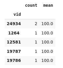

Uh oh, there's a little problem here. There are lots of VNs with top ratings (10) but only as few as 1 votes. Surely they are not the most popular VNs, so how to find the VNs which have high ratings as well as are popular enough to get lots of votes.

The commonly used solution is to use Bayesian Ratings. The basic premise is that more popular VNs should be rated by there true rating, whereas VNs with less votes should be shifted closer to the mean rating of the group. This can be done by adding some number of ratings (C) equal to some predefined mean (m) to the ratings of a VN while calculating it's mean rating. Let's try it out.

# Reading vn data to show
vn = pd.read_sql("SELECT id, title from vn", con=engine)
vn.set_index("id", inplace=True)
vn.head()

C = 500 # variable count
m = 85  # variable mean
best_vns = finished.groupby("vid").agg(["count", "sum", "mean"])["vote"]
best_vns["bayes_rating"] = (C*m + best_vns["sum"])/(C + best_vns["count"])
best_vns.sort_values(by="bayes_rating", ascending=False, inplace=True)
best_vns = best_vns.join(vn, how="left")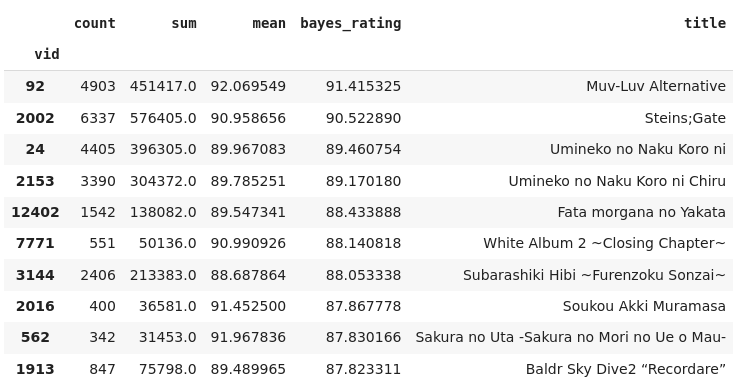

Much better, as it represents the really popular and highly rated VN.

A Content Based model based on Tags

Let's finally get into RecSys territory. Here we will build a simple Content-Based recommendation model using the tags metadata.

In a Content-Based model, we use the item description and metadata to recommend new similar items.

Let's load the relevant data.

# Load vn table
vn = pd.read_sql_table("vn", con=engine)
vn.set_index('id', inplace=True)


# Read tags for every vn and average vote given to that tag (only selected those given positive votes)
tags = pd.read_sql('SELECT tv.vid, tv.tag, t.name, AVG(tv.vote) AS vote FROM tags_vn tv INNER JOIN tags t ON tv.tag = t.id WHERE tv.vote > 0 GROUP BY tv.vid, tv.tag, t.name ORDER BY AVG(tv.vote) DESC;', con=engine)

# Average number of tags per VN
tags.groupby('vid').count()['tag'].describe()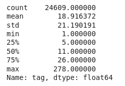

Preprocessing the tags

While building a model, we don't want to bother with the lengthy and irregular tag names themselves, so we can use the tag id to represent the tag associated with a VN.

Morevoer since tags have votes with respect to VNs, to capture this measure, let's repeat a tags according to the number of votes it has. Thus tags having more votes will occur more than those with less votes.

# Instead of using tag names, I'm using tag ids as the tags,
# since they are unique and don't need to be cleaned
tags['tagname'] = tags['tag'].apply(str)

# Populate tags by using vote as frequency
tags['tagvalue'] = np.ceil(tags['vote'] * 10).astype('int') * (tags['tagname'] + ' ')
tags.sample(5)

# Since we are only using tags, we can ignore other columns
# Group all tags by VN
def join_tags(tags):
  return ' '.join(tags)

vn_tags = tags.groupby('vid')['tagvalue'].agg(join_tags)
vn_tags.head()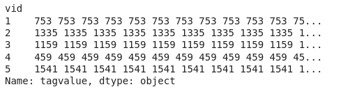

Now we have just the VNs and their tag information. So let's build the model.

Building the model : TF-IDF and Cosine Similarity

First of all, we need to encode the tags. SInce algorithms work better with numbers, encoding does exactly that, convert test data to numbers. There are various ways to do this.

One Hot Encoding
TF-IDF
Word Embeddings

Here we will use TF-IDF.

What is TF-IDF? Term Frequency - Inverse Document Frequency (see why we call it TF-IDF), is used to evaluate how important a word is to a document in a possibly large corpus of words.

The first term TF measures how frequent a word is in a document.
The second IDF term how important a word is overall.

For example, there is a VN with 'adv' and 'baseball' tags. Now the 'adv' adventure tag occurs in a lot of VNs so it is considered less important whereas only a few VNs are related to 'baseball' so baseball, when it occurs is considered more important. This will help us finding similar VNs.

We can easily convert tag data to TF-IDF scores using scikit-learn.

# I am using TF-IDF to parse tag information of VNs
from sklearn.feature_extraction.text import TfidfVectorizer
tfidf = TfidfVectorizer(analyzer='word', ngram_range=(1, 1), token_pattern=r'\S+')

Now how to actually find similar VNs? This can be done using the cosine similarity

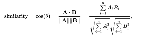
Given two vectors representations, using this formula we can measure the similarity between them. And since we have tag information in form of encoded vectors for all VNs, we just need to use cosine similarity between each pair of VNs.

# Using Cosine Similarity to measure similarity between two VNs
# TF-IDF already applies normalization, so using linear_kernel
from sklearn.metrics.pairwise import linear_kernel
cosine_similarity = linear_kernel(tfidf_matrix, tfidf_matrix)

# Converting to Dataframe for indexing
cosine_similarity = pd.DataFrame(cosine_similarity, index=vn_tags.index, columns=vn_tags.index)

As easy as that!

Now that we have the similarity scores for each pair of VNs, we are ready to make some predictions.

# Make N predictions by finding VNs similar to given VN id
def get_recommendation(vnid, N=5):
  if vnid not in cosine_similarity.index:
    print(f"VN with id {vnid} not present in recommendation engine.")
    return
  sim_scores = cosine_similarity.loc[vnid].sort_values(ascending=False)
  most_similar = sim_scores[1:N+1].index  # ignoring itself
  return vn.loc[most_similar][['title']]

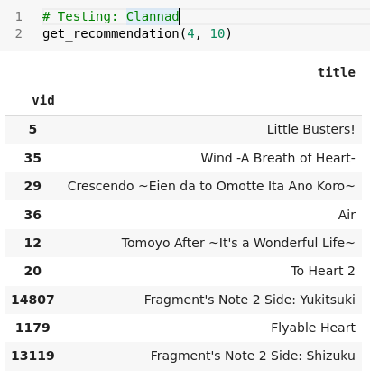
This funtions returns the N most similar VNs to any given VN. Let's try to make some predictions:

Clannad :

Steins;Gate :

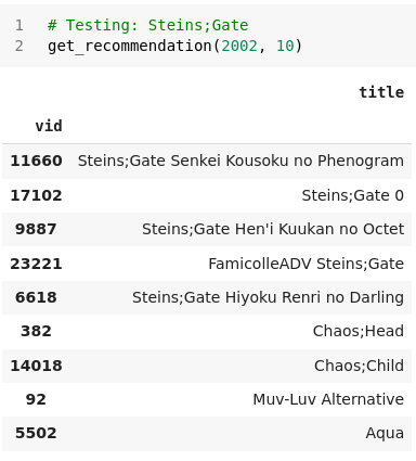
Fate/Stay Night :

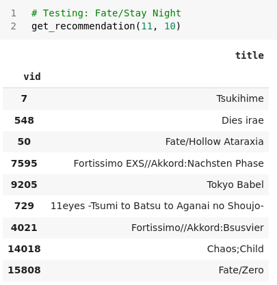
Our model works! And looks pretty good for a simple naive model. Creating this simple model was pretty easy as far as implementation goes. The hard part is understanding the data and the right algorithms to use. Let's gauge the pros and cons of this model.

Advantages:

No need for user data, so does not suffer from sparsity or cold start problems.
Can recommend new and unpopular items.
The recommendations can be explained by showing similar tags.

Disadvantages:

Can't provide personalized recommendations
Unable use quality judgements of users via ratings.

Next up we will work on building memory based collaborative filtering models.

Here are the notebooks with the code : EDA and Content Based Model.

Categories